Introduction

• The goal of this task is to fit a statistical model to historical credit data and then use the model to estimate the value of current loans.

• Since this is a binary classification problem where the target variable is either DEFAULT or PAID, I will use Logistics Regression.

• In addition to model building, I will illustrate how sklearn’s Pipeline is more convenient and simple to use than manually doing all transformation steps - especially for Cross Validation and Hyperparameters Tuning

Data descriptions

Column	account_no
account_no	A unique account number per loan
gender	The gender of the account holder - either "M" or "F"
age	The age of the account holder at the point of application
income	The monthly net income of the account holder at the point of application
loan_amount	The amount of money lent
term	The number of months that the loan is to be repaid over
installment_amount	The monthly installment amount
interest_rate	The interest rate on the loan
credit_score_at_application	The credit score at the point of application, this is a positive integer less than 1000. The higher the score the more creditworthy the applicant is believed to be
outstanding_balance	The remaining amount of the loan that still has to be repaid
status	This indicates what state the account is in. This field can take one of three values - "LIVE" : The loan is still being repaid - the field outstanding_balance will be greater than zero. - "PAID_UP": The loan has been completely repaid - the field outstanding_balance will be zero. - "DEFAULT": The loan was not fully repaid and no further payments can be expected - the field outstanding_balance will be greater than zero and the amount will not be recoverable.

0. Imports and read data

import numpy as np
import pandas as pd
import matplotlib.pyplot as plt
import seaborn as sns

from sklearn.linear_model import LogisticRegression
from sklearn.preprocessing import OneHotEncoder, StandardScaler
from sklearn.metrics import accuracy_score, recall_score, precision_score, f1_score, roc_curve
from sklearn.pipeline import Pipeline
from sklearn.compose import ColumnTransformer
from sklearn.model_selection import train_test_split, cross_val_score, KFold, GridSearchCV

df = pd.read_csv('./data/loan_default.csv')
df.head()

index	account_no	gender	age	income	loan_amount	term	installment_amount	interest_rate	credit_score_at_application	outstanding_balance	status
0	acc_00000316	F	18	12143	47000	60	1045	0.12	860	0	PAID_UP
1	acc_00000422	F	18	6021	13000	60	330	0.18	640	0	PAID_UP
2	acc_00001373	F	39	12832	13000	60	296	0.13	820	0	PAID_UP
3	acc_00001686	F	33	4867	5000	36	191	0.22	540	0	PAID_UP
4	acc_00001733	F	23	5107	22000	36	818	0.20	580	11314	LIVE

1. Exploratory Data Analysis

• account_no column is just an unique identifier and has no predictive power, we will drop it
• outstanding_balance will have value =0 for PAID_UP status. Hence we will need to drop this column as well to prevent data leakage.

1.1 Remove LIVE rows

• As the business goal of this task is to estimate value of current loans, we will drop rows where status column is LIVE.
• We will train the model on terminal loan statuses and run the prediction on this LIVE dataset later.

df_full_train = df.drop(df.loc[df['status']=='LIVE'].index)
df_live = df.loc[df['status']=='LIVE']

The proportion of DEFAULT is about 7%. This level is used to sense check with the final model.

df_full_train['status'].value_counts(normalize=True).round(3)

>>> PAID_UP    0.931
>>> DEFAULT    0.069
>>> Name: status, dtype: float64

Since the target variable is either PAID_UP or DEFAULT, we can simply replace the values. Since we are interested in DEFAULT, I will make it the positive class with value 1

df_full_train['status'] = df_full_train['status'].map({
    'PAID_UP': 0,
    'DEFAULT': 1
})

df_full_train.head()

index	account_no	gender	age	income	loan_amount	term	installment_amount	interest_rate	credit_score_at_application	outstanding_balance	status
0	acc_00000316	F	18	12143	47000	60	1045	0.12	860	0	0
1	acc_00000422	F	18	6021	13000	60	330	0.18	640	0	0
2	acc_00001373	F	39	12832	13000	60	296	0.13	820	0	0
3	acc_00001686	F	33	4867	5000	36	191	0.22	540	0	0
5	acc_00002114	M	38	9328	25000	36	904	0.18	630	0	0

X = df_full_train.drop(['account_no', 'outstanding_balance', 'status'], axis=1)
y = df_full_train['status']

1.2 Univariate distributions of features

NUMERICAL = list(df.select_dtypes(include='number').columns)
CATEGORICAL = list(df.select_dtypes(include='object').columns)
print(NUMERICAL)
print(CATEGORICAL)

>>> ['age', 'income', 'loan_amount', 'term', 'installment_amount', 'interest_rate', 'credit_score_at_application', 'outstanding_balance']
>>> ['account_no', 'gender', 'status']

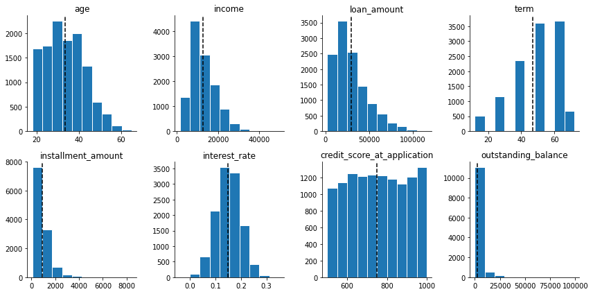
To understand the distributions of numerical data, we can plot individual historgrams

• Since I want to interpret the coefficients, I will just leave them as is for the base model instead of transforming.
• For this dataset, we don’t have issue with outliers except for outstanding_balance. But we will not be using this feature anyway.

fig, axes = plt.subplots(2, 4, figsize=(12, 6))

for idx, col_name in enumerate(NUMERICAL):
    ax = axes[idx//4, idx%4]
    ax.set_title(col_name)
    ax.hist(df[col_name], ec='white')
    ax.axvline(x=df[col_name].mean(), ls='--', color='k')
    sns.despine(ax=ax)

fig.tight_layout()

1.3 Bivariate relationship between features and target variable

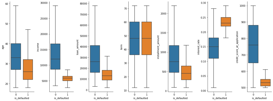
• To understand the relationship between each individual feature with the target, we can plot a correlation chart. However, since the target is binary, I will use boxplot instead.
• In the charts below, income, interest_rate and credit_score_at_application are the strongest predictors of whether the loanee will default.

fig2, axes2 = plt.subplots(1, len(NUMERICAL[:-1]), figsize=(16, 6))

for idx, col_name in enumerate(NUMERICAL[:-1]):
    sns.boxplot(
        df_full_train[[col_name, 'status']],
        x='status',
        y=col_name,
        showfliers=False,
        ax=axes2[idx])
    
    axes2[idx].set_xlabel('is_defaulted')
    sns.despine(ax=axes2[idx])

fig2.tight_layout()

2. Manual fitting

X_train, X_test, y_train, y_test = train_test_split(X, y, test_size=0.2, random_state=1)

X_train = X_train.reset_index(drop=True)
X_test = X_test.reset_index(drop=True)

y_train = y_train.reset_index(drop=True)
y_test = y_test.reset_index(drop=True)

2.1 Preprocessing

2.1.1 Check for NaN/Nulls values

X_train.isnull().sum()

>>> gender                         0
    age                            0
    income                         0
    loan_amount                    0
    term                           0
    installment_amount             0
    interest_rate                  0
    credit_score_at_application    0
    dtype: int64

2.1.2 Categorical data

We will use one-hot encoding for gender. 0 represents Female, 1 represents Male

gender_encoder = OneHotEncoder(drop='first')
gender_encoder.fit(X_train['gender'].values.reshape(-1, 1))
gender_encoder.categories_

>>> [array(['F', 'M'], dtype=object)]

# encode column
encoded_gender = gender_encoder.transform(X_train['gender'].values.reshape(-1, 1)).toarray()

# convert encoded columns into dataframe
encoded_gender_df = pd.DataFrame(
    encoded_gender,
    columns=gender_encoder.get_feature_names_out()
)

# merge original df with encoded df
X_train = pd.concat(
    [X_train, encoded_gender_df],
    axis=1,
)

# drop original column
X_train = X_train.drop(['gender'], axis=1)

X_train.head()

index	age	income	loan_amount	term	installment_amount	interest_rate	credit_score_at_application	x0_M
0	33	16685	55000	60	1223	0.12	850	1.0
1	27	15050	28000	24	1331	0.13	840	1.0
2	50	40203	62000	48	1345	0.02	1000	1.0
3	26	13754	39000	48	1066	0.14	810	1.0
4	30	11830	31000	60	705	0.13	810	0.0

2.1.3 Numerical data

For the base model, we keep numerical data intact.

2.2 Fitting Logistics Regression Model

log_reg = LogisticRegression(max_iter=1_000)
log_reg.fit(X_train, y_train)

LogisticRegression(max_iter=1000)

In a Jupyter environment, please rerun this cell to show the HTML representation or trust the notebook.
On GitHub, the HTML representation is unable to render, please try loading this page with nbviewer.org.

2.3 Model coefficients

An advantage of Logistics Regression is that the coefficients are white box, making it easier for stakeholders to understand why the model makes a certain prediction.

We can write the full formula based on the fitted model’s intercept and coefficients

log_reg.intercept_
>>> array([1.22179855])

model_coefficients = dict(zip(
    list(log_reg.feature_names_in_),
    list(log_reg.coef_[0]))
    )

model_coefficients

>>> {'age': 0.057494705504614954,
     'income': -0.0032484557471085074,
     'loan_amount': -2.8753044215366256e-05,
     'term': 0.022543857502140222,
     'installment_amount': 0.0009745065842801654,
     'interest_rate': 0.6331692246041164,
     'credit_score_at_application': 0.0165512445820803,
     'x0_M': 7.976349551593769}

Hence the full formula is:

\[z = 1.222 + age * 0.057 +income * -0.003 +loan\_amount * -0.0 +term * 0.023 +installment\_amount * 0.001 +interest\_rate * 0.633 +credit\_score\_at\_application * 0.017 +x0\_M * 7.976\] \[prob(default) = \frac{1}{1 + e^{-z}}\]

To make a sample prediction, we can apply the above formula as follow:

sample_data = {
    'age': 30,
    'income': 10_000,
    'loan_amount': 20_000,
    'term': 60,
    'installment_amount': 1_000,
    'interest_rate': 0.15,
    'credit_score_at_application': 800,
    'x0_M': 1,
}


def sigmoid(n):
    return 1 / (1 + np.e ** (-n))

z = 1.22179855 + (np.array(list(model_coefficients.values())) * np.array(list(sample_data.values()))).sum()

print('probability of default for sample data')
print(sigmoid(z))
>>> probability of default for sample data
>>> 0.0015414024478882305

To verify that the function works, we can compare predicted default probability by using the model’s .predict() method

>>> log_reg.predict_proba(np.array(list(sample_data.values())).reshape(-1, 8))[:, 1][0]
>>> 0.0015414024462043266

2.4 Making predictions

Now that we understand how the model works, let’s see how it performs on test data.

In order to run the model on test data, we need to perform the same transformation steps above.

# encode column
encoded_gender = gender_encoder.transform(X_test['gender'].values.reshape(-1, 1)).toarray()

# convert encoded columns into dataframe
encoded_gender_df = pd.DataFrame(
    encoded_gender,
    columns=gender_encoder.get_feature_names_out()
)

# merge original df with encoded df
X_test = pd.concat(
    [X_test, encoded_gender_df],
    axis=1,
)

# drop original column
X_test = X_test.drop(['gender'], axis=1)
X_test.head()

index	age	income	loan_amount	term	installment_amount	interest_rate	credit_score_at_application	x0_M
0	37	14163	28000	60	652	0.14	780	1.0
1	27	10769	33000	24	1584	0.14	790	0.0
2	28	10747	34000	48	929	0.14	790	0.0
3	22	14439	49000	24	2284	0.11	910	0.0
4	32	6400	17000	36	649	0.22	540	1.0

y_preds = log_reg.predict(X_test)
y_preds
>>> array([0, 0, 0, ..., 0, 0, 0])

2.5 Evaluate model

Accuracy, Recall, Precision, f1-score

def evaluate_model(y_true, y_pred):    
    result = {
        'accuracy': accuracy_score(y_true, y_pred),
        'recall': recall_score(y_true, y_pred),
        'precision': precision_score(y_true, y_pred),
        'f1_score': f1_score(y_true, y_pred),
    }

    return result

evaluate_model(y_test, y_preds)
>>> {'accuracy': 0.9705,
>>> 'recall': 0.8035714285714286,
>>> 'precision': 0.8385093167701864,
>>> 'f1_score': 0.8206686930091185}

ROC curve

fpr, tpr, thres = roc_curve(y_test, log_reg.predict_proba(X_test)[:, 1])

fig, ax = plt.subplots()
ax.set_aspect(1)
ax.plot(fpr, tpr, label='logistics regression model')
ax.plot(np.linspace(0, 1, 1_000), np.linspace(0, 1, 1_000), ls='--', label='random guess')
ax.legend()
ax.set_xlabel('False positive rate')
ax.set_ylabel('True positive rate')

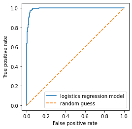
At this point we have a working model.

However in practice we rarely build just 1 model. We will need to experiment with different types of tranformation, and tuning hyperparameters

As the number of transformations and parameters increases, we will need to keep track of more objects. This is cumbersome and prone to error. That’s why we will use a Pipeline.

3. Using Pipelines

We can build the same model as above using fewer lines of code thanks to Pipeline

X_train, X_test, y_train, y_test = train_test_split(X, y, test_size=0.2, random_state=1)

X_train = X_train.reset_index(drop=True)
X_test = X_test.reset_index(drop=True)

y_train = y_train.reset_index(drop=True)
y_test = y_test.reset_index(drop=True)

3.1 Column transformers

# define the column transformer to encode gender column
column_transformer = ColumnTransformer(
    transformers=[
        ('encoder', OneHotEncoder(drop='first'), ['gender'])
    ],
    remainder='passthrough'
)

3.2 Build and fit pipeline

# define the pipeline with column transformer and logistic regression
pipeline = Pipeline([
    ('preprocessor', column_transformer),
    ('classifier', LogisticRegression(max_iter=1_000))
])

# fit the pipeline to the training data
pipeline.fit(X_train, y_train)

preds = pipeline.predict(X_test)

evaluate_model(y_test, preds)
>>> {'accuracy': 0.9705,
>>> 'recall': 0.8035714285714286,
>>> 'precision': 0.8385093167701864,
>>> 'f1_score': 0.8206686930091185}

Here we can verify that pipeline produces the same result as manual steps by comparing predicted output and metrics.

3.3 Cross validation with Pipeline

• Cross-validation is a technique that is used to evaluate the performance of the model. In cross-validation, the data is split into k-folds, where each fold is used for testing at least once. For example, if 5-fold cross-validation is used, then in the first iteration, fold 1 may be used for testing and folds 2–5 for training. In the second iteration, fold 2 may be used for testing, the rest of the folds for training the model, and so on until all the folds are used for testing at least once.

• K-fold cross-validation can be especially useful when the dataset is small or imbalanced, as it allows for the model to be evaluated on all of the data, even if some observations have low representation in the dataset.

# Define the cross-validation strategy
cv = KFold(n_splits=10, shuffle=True, random_state=42)

# Perform cross-validation
acc_scores = cross_val_score(pipeline, X_train, y_train, cv=cv)

# Compute the mean and standard deviation of the scores
print("Accuracy: %0.2f (+/- %0.2f)" % (acc_scores.mean(), acc_scores.std() * 2))
>>> Accuracy: 0.97 (+/- 0.02)

3.4 Hyperparameters tuning

Hyperparameter tuning refers to the process of selecting the best hyperparameters for a machine learning model in order to achieve optimal performance. In the case of logistic regression classification, hyperparameters are values that are set before the learning process begins and affect the behavior of the model.

Here are some hyperparameters that we can tune for Logistics Regression:

• Regularization strength: Regularization helps to prevent overfitting of the model by penalizing large coefficients. The regularization strength hyperparameter controls the amount of penalization applied.

• Solver: The solver is the algorithm used to optimize the logistic regression objective function. There are several solvers available, such as ‘newton-cg’, ‘lbfgs’, and ‘liblinear’, each with different strengths and weaknesses.

• Maximum number of iterations: The maximum number of iterations determines the maximum number of iterations for the solver to converge.

column_transformer = ColumnTransformer(
    transformers=[
        ('categorical_encoder', OneHotEncoder(drop='first'), ['gender']),
        ('numerical_scaler', StandardScaler(), NUMERICAL[:-1])

    ],
    remainder='passthrough'
)

my_pipeline = Pipeline([
    ('preprocessor', column_transformer),
    ('classifier', LogisticRegression(max_iter=10_000))
])


# Define the hyperparameters to tune
parameters = {
    'preprocessor__numerical_scaler__with_mean': [True, False],
    'classifier__penalty': ['l1', 'l2'],
    'classifier__C': [0.1, 1, 10],
    'classifier__solver': ['liblinear', 'saga']
}


# Create a grid search object
grid_search = GridSearchCV(my_pipeline, parameters, cv=5, verbose=1)


# Fit the grid search object on the data
grid_search.fit(X_train, y_train)

print("Best parameters: ", grid_search.best_params_)
print("Best cross-validation score: ", grid_search.best_score_)

>>> Best parameters:  {'classifier__C': 1, 'classifier__penalty': 'l1', 'classifier__solver': 'saga', 'preprocessor__numerical_scaler__with_mean': True}
>>> Best cross-validation score:  0.9728653846153847

3.5 Retrain piepline on the best params

Training the model on the best params give us improved metrics

column_transformer = ColumnTransformer(
    transformers=[
        ('categorical_encoder', OneHotEncoder(drop='first'), ['gender']),
        ('numerical_scaler', StandardScaler(with_mean=True), NUMERICAL[:-1])

    ],
    remainder='passthrough'
)

best_pipeline = Pipeline([
    ('preprocessor', column_transformer),
    ('classifier', LogisticRegression(penalty='l1', C=1, max_iter=6_000, solver='saga'))
])


# fit the pipeline to the training data
best_pipeline.fit(X_train, y_train)

preds = best_pipeline.predict(X_test)

evaluate_model(y_test, preds)

>>> {'accuracy': 0.971,
>>> 'recall': 0.8214285714285714,
>>> 'precision': 0.8313253012048193,
>>>'f1_score': 0.8263473053892216}

4. Predict model on LIVE loans data

df_live = df_live.drop(['account_no', 'status'], axis=1)
df_live = df_live.reset_index(drop=True)
df_live['predicted_default'] = best_pipeline.predict(df_live.drop(['outstanding_balance'], axis=1))
df_live['default_prob'] = best_pipeline.predict_proba(df_live.drop(['outstanding_balance'], axis=1))[:, 1].round(3)

df_live.head()

index	gender	age	income	loan_amount	term	installment_amount	interest_rate	credit_score_at_application	outstanding_balance	predicted_default	default_prob
0	F	23	5107	22000	36	818	0.20	580	11314	0	0.043
1	F	40	15659	33000	48	853	0.11	880	5637	0	0.000
2	M	25	15660	15000	48	395	0.12	860	6039	0	0.000
3	F	30	4208	15000	48	481	0.23	530	2817	0	0.297
4	F	18	6535	12000	48	346	0.17	660	3120	0	0.001

expected_book_value = (df_live['outstanding_balance'] * (1 - df_live['default_prob'])).sum()
print(f"total outstanding balance =\t{df_live['outstanding_balance'].sum():,.2f}")
print(f"expected recoverable value =\t{expected_book_value:,.2f}")

>>> total outstanding balance =	24,622,111.00
>>> expected recoverable value = 23,809,056.25

5. Summary

What we did

• We built a Logistics Regression for a classification of loan default.
• We chose Logistics Regression because it’s a white box model with clear parameters, making iteasier to explain to business stakeholders.
• We used sklearn’s Pipeline to make it easy to do Cross Validation and Hyperparameters Tuning

Improvement ideas

• For the sake of simplicity I have not factored in time value of money. But this can be done by discounting each payment according to their expected due date.
• By default, pipeline.predict() has a decision threshold of 0.5. Meaning that if pipeline.predict_proba() is above 0.5 then the data will be classified as default.
  • At a recall score of 0.82 we expect about 8 out of 10 defaults are identified.
  • We can improve recall by lowering the decision threshold. The cost will be more false positive (non-default classified as default)
  • Depending on the business objective, we can fine tune threshold level. If we want to be conservative with our estimate, then higher recall might be more acceptable.
• We can also explore ensemble methods, such as xgboost, as it works well with tabular data