Introduction

Cohort analysis provides insights into users behaviors by segmenting them into mutually exclusive groups and observe the differences. Though there are multiple ways to define a cohort, the most common is grouping users by acquisition date.

Most serious analytics software have built-in cohort analysis tools. But knowing how to create one using python can come in handy.

Creating a cohort heatmap

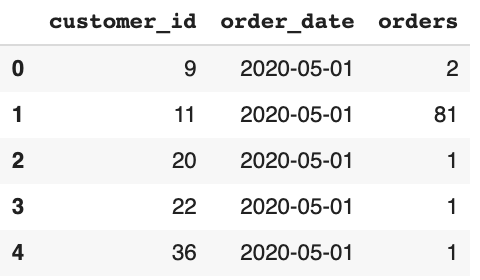
Input data is a generic sales log including 3 columns: unique customer id, order date and orders quantity

df.head()

The most suitable time range depends on your product: the choice could be day/week/month. For an apps that you expect daily user (such as a language learning apps, daily frequency is suitable). For an e-commerce website, perhaps monthly purchases would yield the best indicator.

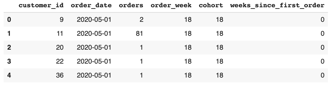
df['order_week'] = df['order_date'].dt.isocalendar().week
df['cohort'] = df.groupby('customer_id')['order_week'].transform('min')
df['weeks_since_first_order'] = df['order_week'] - df['cohort']

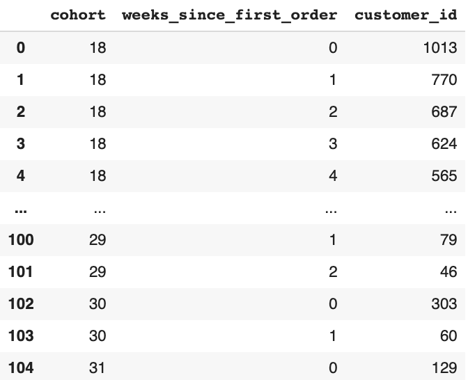
cohort_data = df.groupby(['cohort', 'weeks_since_first_order'])['customer_id'].apply(pd.Series.nunique).reset_index()
cohort_data.head()

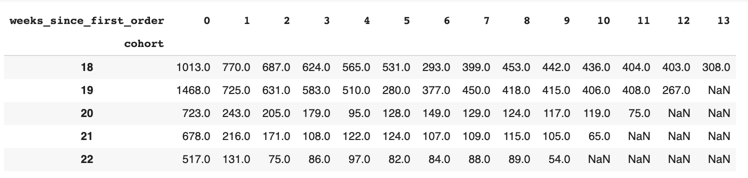
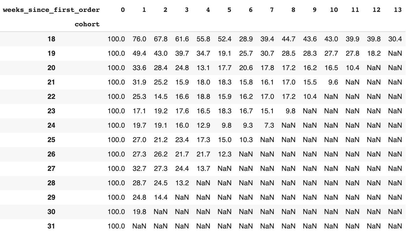
cohort_count = cohort_data.pivot_table(index='cohort',
                                       columns='weeks_since_first_order',
                                       values='customer_id')
cohort_count.head()

retention = cohort_count.divide(cohort_count.iloc[:,0], axis=0).round(3) * 100

Plotting cohort using seaborn

fig, ax = plt.subplots(figsize=(15,6))
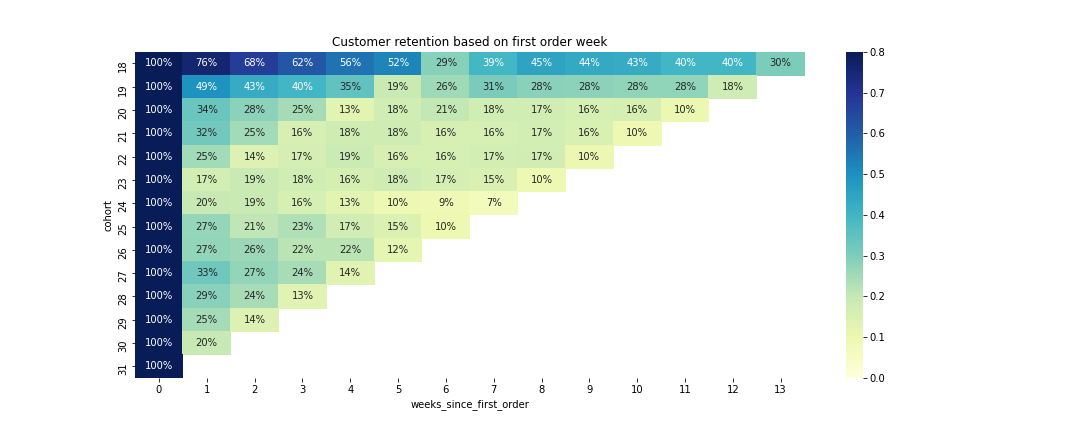
ax.set_title('Customer retention based on first order week')
sns.heatmap(data=retention,
            annot=True,
            fmt = '.0%',
            vmin=0,
            vmax=.8,
            cmap='YlGnBu', ax=ax)

fig.savefig('retention-heatmap.png', transparent=True)

Using cohort heatmap

Each row of the chart corresponds to a temporal cohort. The first column is always equal to 100% because, and subsequnt columns shows that percentage of that cohort remaning after a given period of time.

• Horizontal features identify a cohort-specific trait. For example, if you were to run an ad campaign in a given week, you might see a horizontal feature emerge showing improved or dimished retentino particular to that cohort. In the heatmap, week 24 cohort has significantly lower retention than the neighboring weeks. By week 6, less than 10% of the cohort remained.
• Diagonal features are usually the results of product or performance changes. The first few weeks from week 18 to 22 tends to have greater retention than the later weeks. This might indicate that product quality might have been deteriorating.
• Vertical features are commonly seens in subcription services. For example, a dollar chart might show a significant feature every 12 months when portions of cohorts renew their memership.

Since total retention is the weighted average of cohort retentions, it is important to track cohorts that are much greater than others.

End