Simulating a queue system
Introduction
In this post I will use simpy to simulate a queueing line at the airport check in counters. This is an example of Discret-event simulation (DES). In contrast to Monte-Carlo simulation, DES are useful when you need to keep track of a system’s state and analyze resource usage over time.
There are many practial use cases where you might need DES. In particular, for a queue system, we want to balance out cost (as reflected by number of counters) vs. customer experience (as measured by wait time)
 Picture I took at Changi Airport before going on a vacation
Assumptions & Methodology
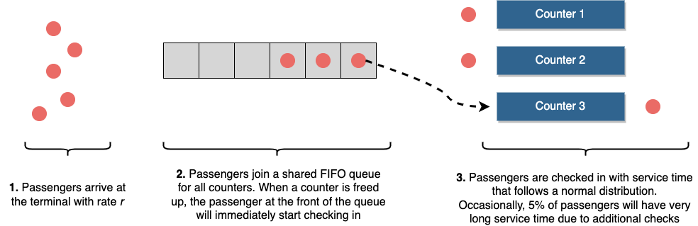
- There are 8 counters available for check-in. When passengers arrive that the airport terminal, they will join a shared queue and go up to the next available counter.
- Check-in time follows a normal distribution with a mean of 2 minutes and standard deviation of 1 minute. To spice things up, I’ve also added a 5% chance that a passenger might have issues with their paperwork and can take up to 10 minutes to resolve.
- Before the counter opens, a group of 30 passengers arrived at the airport. (They just want to have more buffer time and enjoy walking around the airport)
- In the first 30 minutes, passengers arrive at a slower rate. Afterwards, the arrival rate increases.
The above assumptions are coded as following:
NUM_COUNTERS = 8

CHECK_DURATION_AVG = 2
CHECK_DURATION_STD = 1

PASSENGER_INTERVAL_1ST = 1 # on average, 1 customer arrived every minute
PASSENGER_INTERVAL_2ND = .33 # on average, 3 customers arrived every minute

INITIAL_NUM_PASSENGERS = 30
MAX_PASSENGERS = 250
Note: In simpy, time units can be arbitrary depending on the problem you are modeling. For the sake of clarify, I will use minutes to measure time in this model.
The full code can be found at the end of the post. Here I’d like to highlight a few key details:
Modeling the check in process
def check_in(self, passenger):

    p = np.random.uniform(low=0.0, high=1.0)

    # normal passengers
    if p < .95:
        random_time = max(1, np.random.normal(self.check_duration, self.check_std))

    # 5% of passengers have problems and need more time
    else:
        random_time = max(10, np.random.normal(self.check_duration, self.check_std))

    print(f'Start checking in passenger {passenger} at {self.env.now:1f}')
    yield self.env.timeout(random_time)
    print(f'Finish checking in passenger {passenger} at {self.env.now:1f}')
Here we’re doing 2 things:
p = np.random.uniform(low=0.0, high=1.0)
if p < .95:
    ...
We get a random number, if the value is < .95, then the passenger’s check in time follows the distribution with CHECK_DURATION_AVG and CHECK_DURATION_STD. For the remaining 5% of the cases, the staff will need 10 minutes to complete.
print(f'Start checking in passenger {passenger} at {self.env.now:1f}')
yield self.env.timeout(random_time)
print(f'Finish checking in passenger {passenger} at {self.env.now:1f}')
This is the actual check-in event. The 2 printing functions are optional, but helpful to collect the output to analyze the system. The env.timeout() method simulates check-in duration.
Modeling passengers behavior
def passenger(env, pid, ch_in):
    """
    pid = unique identifier for passenger
    """
    print(f'Passenger {pid} arrived at the airport and join the queue at {env.now:.1f}')

    # join queue and wait for the next available counter
    with ch_in.staff.request() as request:
        yield request
        yield env.process(ch_in.check_in(pid))
This is the passenger process. Each passenger is assigned a unique id (pid) for ease of tracking.
with ch_in.staff.request() as request:
    yield request
    yield env.process(ch_in.check_in(pid))
This part simulates the passenger joining the queue, and will be served when they’re at the front of the queue and there’s an available counter.
Setting up the simulation
def setup(env, initial_passengers, passenger_interval_1st, passenger_interval_2nd, max_passengers):
    # initialize first of group passengers who arrived before counter open
    for i in range(initial_passengers):
        env.process(passenger(env, i, ch_in))


    # simulate passengers coming in with normal interarrival time
    while i <= max_passengers:
        # first hour
        if env.now < 30:
            t = np.random.exponential(passenger_interval_1st)

        else:
            t = np.random.exponential(passenger_interval_2nd)

        yield env.timeout(t)

        i += 1
        env.process(passenger(env, i, ch_in))
Normally, we don’t run the simulation just once and take the first result! But instead we will repeat it for ten or hundred of thousand times and perhaps changing the assumptions/parameters. Hence it’s convenient to write a setup function to initialize the simulation.
The rest of the codes are standard python functions. You can add additional logging features to help debug or customize queue logic.
Results & Observations
Passengers arrival
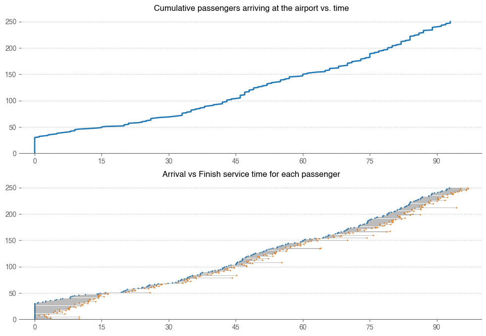 Fig 1 (top), Fig 2 (bottom)
Figures 1 and 2 shows details for individual passengers.
- Figure 1 shows the cumulative number of passengers arriving against time
- At time 0, we had 30 passengers before the counters opended. The line starts at point (0, 30).
- The slope is flatter before the 30 minutes mark, and got stepper afterwards. This is because we assumed higher arrival rate.
- Figure 2 shows the time each passenger spent in the queue system: from arriving at the terminal until they finished checking in
- Each passenger is one horizontal line. The blue dots indicate start time, orange dots indicate end time.
- The length of the line is proportional to the time taken.
- The longer lines that stand out incidate passengers with issues and held their counter up for 10 minutes ;(
- Additional details for wait time
| service_time | |
|---|---|
| count | 250 |
| mean | 2.55555 |
| std | 2.00238 |
| min | 1 |
| 25% | 1.4025 |
| 50% | 2.07835 |
| 75% | 2.91865 |
| max | 10 |
Queue and Utilization
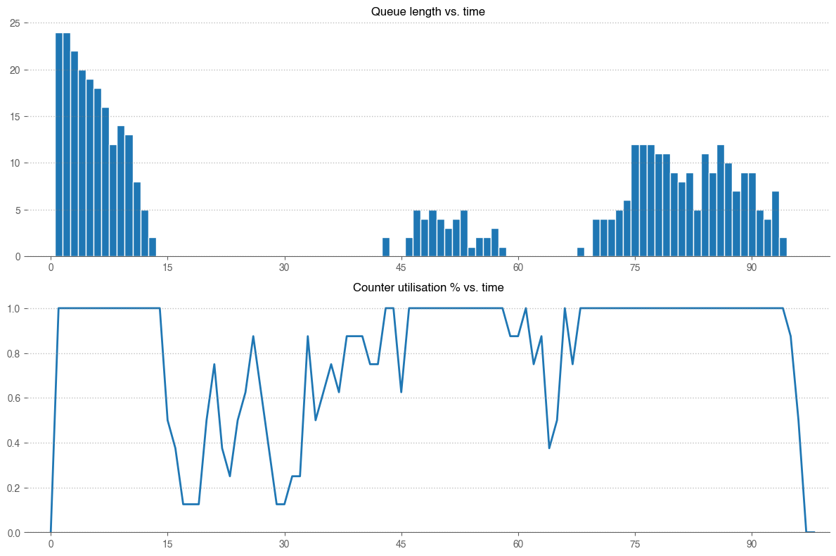 Fig 3 (top), Fig 4 (bottom)
Figure 3 and 4 monitor queue length and resource utilizations.
- In Figure 3, we can see the queue line is the longest at the beginning
- This is due to the group of early passengers. Therefore, if you don’t want to wait in line, it’s probably best to avoid arriving too early!
- The queue starts to build up again as passengers arrived at an increased rate after 30 mins.
- Finally we are also interested in resource utilizations. This is where the trade-off comes in.
- Utilization at any time is measured as the number of busy counter / total number of counters
- We can estimate overall utilization by measuring area under the curve. In this case it’s equal to roughly 81%
- As a business owner, we wouldn’t want our resources to stay idle for too long. Perhaps we might try to reduce the number of counter by 1 and re-run the simulation. However, it’s important to note that for an airport, all passengers need to be checked-in before flight time. Hence maximum utilization might not be the highest priority.
Takeaway
- This is only a toy sample with somewhat simple assumptions. We can observe real data and model the different processes (arrival time, check-in time, etc) more accurately. However, even with such simple assumptions, we can see that DES is an useful tool for analyzing systems and finding bottlenecks.
- For our airport queue model, we only take number of counters as cost. However, in another business scenario (such as a restaurant queue), costs might also include lost income from reneged customer (who might wait too long).
- Simpy is flexible and not just limited to modelling queueing. Other use cases might be allocating production capacity at a manufacturing plant, or perhaps scheduling transportation trucks between warehouses. All these real life scenarios inherently contains a lot of random variations and would benefit from DES.